using Makie, MakieRecipes

The simplest example model

using MakieRecipes.RecipesBase

struct T end

RecipesBase.@recipe function plot(::T, n = 1; customcolor = :green)
    markershape --> :auto        # if markershape is unset, make it :auto
    markercolor :=  customcolor  # force markercolor to be customcolor
    xrotation   --> 45           # if xrotation is unset, make it 45
    zrotation   --> 90           # if zrotation is unset, make it 90
    rand(10,n)                   # return the arguments (input data) for the next recipe
end

recipeplot(T(); seriestype = :path)

AbstractPlotting.save("basic.svg", AbstractPlotting.current_scene()); nothing #hide

Testing out series decomposition

sc = Scene()
recipeplot!(sc, rand(10, 2); seriestype = :scatter)
recipeplot!(sc, 1:10, rand(10, 1); seriestype = :path)

AbstractPlotting.save("series.svg", AbstractPlotting.current_scene()); nothing #hide

Differential Equations

using OrdinaryDiffEq, StochasticDiffEq, DiffEqNoiseProcess

A simple exponential growth model

f(u,p,t) = 1.01.*u
u0 = [1/2, 1]
tspan = (0.0,1.0)
prob = ODEProblem(f,u0,tspan)
sol = solve(prob, Tsit5(), reltol=1e-8, abstol=1e-8)

recipeplot(sol)

AbstractPlotting.save("exp.svg", AbstractPlotting.current_scene()); nothing #hide

Matrix DiffEq

A  = [1. 0  0 -5
      4 -2  4 -3
     -4  0  0  1
      5 -2  2  3]
u0 = rand(4,2)
tspan = (0.0,1.0)
f(u,p,t) = A*u
prob = ODEProblem(f,u0,tspan)
sol = solve(prob, Tsit5(), reltol=1e-8, abstol=1e-8)

recipeplot(sol)

AbstractPlotting.save("mat.svg", AbstractPlotting.current_scene()); nothing #hide

Stochastic DiffEq

f(du,u,p,t) = (du .= u)
g(du,u,p,t) = (du .= u)
u0 = rand(4,2)

W = WienerProcess(0.0,0.0,0.0)
prob = SDEProblem(f,g,u0,(0.0,1.0),noise=W)
sol = solve(prob,SRIW1())

recipeplot(sol)

AbstractPlotting.save("stochastic.svg", AbstractPlotting.current_scene()); nothing #hide

Animating a differential equation solution

You can update arguments and attributes arbitrarily, and the recipe pipeline is rerun.

function lorenz(du, u, p, t)
    du[1] = p[1]*(u[2]-u[1])
    du[2] = u[1]*(p[2]-u[3]) - u[2]
    du[3] = u[1]*u[2] - p[3]*u[3]
end

prob = ODEProblem(lorenz, [1., 5., 10.], (0., 100.), (10.0, 28.0, 8/3))

ρ = Node(28.0)

sol = @lift solve(remake(prob; p = (10.0, $ρ, 8/3)), Tsit5())

sc = recipeplot(sol)

ylims!(sc, -30, 70) # avoid jitter when animating

record(sc, "lorenz.gif", LinRange(0, 35, 100)) do ρᵢ
    ρ[] = ρᵢ
end

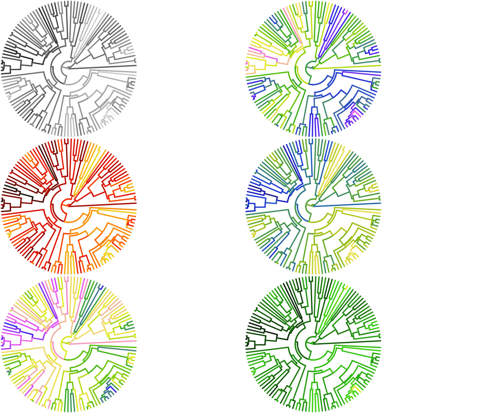
Phylogenetic tree

using Phylo

assetpath = joinpath(dirname(pathof(MakieRecipes)), "..", "docs", "src", "assets")
hummers = open(t -> parsenewick(t, NamedPolytomousTree), joinpath(assetpath, "hummingbirds.tree"))

evolve(tree) = Phylo.map_depthfirst((val, node) -> val + randn(), 0., tree, Float64)

trait = evolve(hummers)

scp = recipeplot(
    hummers;
    treetype = :fan,
    line_z = trait,
    linewidth = 5,
    showtips = false,
    cgrad = :RdYlBu,
    seriestype = :path,
    scale_plot = false, # Makie attributes can be used here as well!
    show_axis = false
)

WARNING: using Phylo.Node in module ex-examples conflicts with an existing identifier.

Animation with different colormaps (changing attributes)

You can update arguments and attributes arbitrarily, and the recipe pipeline is rerun.

record(scp, "phylo_colormaps.gif", PlotUtils.cgradients(:colorcet), framerate = 3) do cmap
    scp.plots[1].cgrad[] = cmap
end

"phylo_colormaps.gif"

GraphRecipes

using GraphRecipes
using GraphRecipes: GraphPlot

In tis case, we don't need access to all of the functions which GraphRecipes provides - just the GraphPlot struct, which is used for recipe dispatch. The rest is handled by the GraphRecipes internals.

The simplest graph recipe

Because userplot is unsupported, we have to use the low-level interface to user plot recipes, by wrapping our arguments in the userplot type. Arguments must be supplied as a Tuple or some other iterable.

recipeplot(
    GraphPlot(
        (
        [0  1  1;
         1  0  1;
         1  1  0],
         )
    );
    show_axis = false,
    scale_plot = false
)

AbstractPlotting.save("simplegraph.svg", AbstractPlotting.current_scene()); nothing #hide

Undirected graph with node labels and sizes

n = 15
A = Float64[ rand() < 0.5 ? 0 : rand() for i=1:n, j=1:n]
for i=1:n
    A[i, 1:i-1] = A[1:i-1, i]
    A[i, i] = 0
end

recipeplot(
        GraphPlot((A,));
        markersize = 0.2,
        node_weights = 1:n,
        markercolor = range(colorant"yellow", stop=colorant"red", length=n),
        names = 1:n,
        fontsize = 10,
        linecolor = :darkgrey,
        show_axis = false,
        scale_plot = false
    )

AbstractPlotting.save("undigraph.svg", AbstractPlotting.current_scene()); nothing #hide

Multigraphs

recipeplot(GraphPlot(([[1,1,2,2],[1,1,1],[1]],)); names="node_".*string.(1:3), nodeshape=:circle, self_edge_size=0.25, show_axis = false, scale_plot = false)

AbstractPlotting.save("digraph.svg", AbstractPlotting.current_scene()); nothing #hide

Julia AST

code = quote
    function mysum(list)
        out = 0
        for value in list
            out += value
        end
        out
    end
end

recipeplot(code; fontsize = 12, shorten = 0.01, axis_buffer = 0.15, nodeshape = :rect)
AbstractPlotting.save("ast.svg", AbstractPlotting.current_scene()); nothing #hide

Type tree with GraphRecipes

recipeplot(AbstractFloat; method = :tree, fontsize = 10)
AbstractPlotting.save("typetree.svg", AbstractPlotting.current_scene()); nothing #hide

This page was generated using Literate.jl.